Misleading the Public for Fun and Profit

Sometimes I read a research paper, usually in the area where computer science meets application, and it’s obvious that the authors are far overstating the practical impact of the work. This can be due to the researchers simply not having any exposure to the practical side of the field in which they are investigating and thus accidentally (through ignorance) overstate their claims. Alternatively it can be a purposeful and deliberate attempt to mislead and posture in front of a readership that hopefully won’t know any better.

The first case is presumably simple ignorance but is still lamentable. The obvious solution here is to avoid making such claims at all. If the research cannot stand on its own then perhaps it is not worthwhile? Researchers (both academic and industrial) have a habit of jumping on problems they underestimate, throwing a variety of techniques at them, hoping one sticks and then calling the problem solved. This typically occurs when they are not actually required to solve the problem correctly and robustly but merely as a ‘prototype’. They then get pilloried by anyone who actually has to solve the problem properly and almost always because of a disparity between claims made and the real impact rather than issues with methodology, recording or technical aspects.

The second case is far more insidious and unfortunately I think not uncommon. In academic research it can be easy to impress by combining cutting edge, but not necessarily original, research with a practical problem, sort-of solving parts of it and like before declaring it solved. Often followed quickly by phrases involving ‘game changing’, ‘paradigm shifting’ and so forth. Personally, I think this is a serious problem in the research areas that are less theoretical and more practical. Often the investigators refuse to accept they aren’t actually aware of the true nature of the problem they are dealing with or how it occurs in the real world. Egotistically this is difficult as they are often lauded by their academic peers and therefore surely must grasp the trivialities of the practical world, no? At this point a mixture of ego, need to impress and lack of ethics combine to give us papers that are at best deluded and at worst downright wrong.

Regardless of whether a paper ends up making such claims mistakenly for the first or the second reason the result is the same. It cheapens the actual value of the research, results in a general loss of respect for the capabilities of academia, deludes the researchers further and causes general confusion as to where research efforts should be focused. Worse still is when attempts to overstate the impact are believed by both the media and other researchers resulting in a complete distortion between the actual practical and theoretical value of the research and it’s perceived impact.

Now, on to the paper that has reminded me of this most recently: The latest paper from David Brumleys group at CMU titled AEG: Automatic Exploit Generation. I was looking forward to reading this paper as it was the area I worked on during my thesis but quite honestly it’s incredibly disappointing at best and has serious factual issues at worst. For now let’s focus on the topic at hand ‘overstating the impact of academic research cheapens it and spreads misinformation‘. With the original Patch-Based Exploit Generation paper we had all sorts of stories about how it would change the way in which patches had to be distributed, how attackers would be pushing buttons to generate their exploits in no time at all and in general how the world was about to end. Naturally none of this happened and people continued to use PatchDiff. Unfortunately this is more of the same.

Near the beginning of the most recent paper we have the following claim “Our automatic exploit generation techniques have several immediate security implications. First, practical AEG fundamentally changes the perceived capabilities of attackers“. This statement is fundamentally flawed. It assumes that practical AEG is currently possible on bugs that people actually care about. This is patently false. I’ve written one of these systems. Did it generate exploits? Yes it did. Is it going to pop any program running on a modern operating system with the kinds of vulnerabilities we typically see? Nope. That would require at a minimum another 2 years of development and at that point I would expect a system that is usable by a skilled exploit writer as an augmentation of his skillset rather than a replacement. The few times I did use the tool I built for real exploits it was in this context rather than full blown exploit generation. The system discussed in the mentioned paper has more bells and whistles in some areas and is more primitive in others and it is still an unfathomable distance from having any impact on a realistic threat model.

Moving on, “For example, previously it has been believed that it is relatively difficult for untrained attackers to find novel vulnerabilities and create zero-day exploits. Our research shows this assumption is unfounded“. It’s at this point the distance between the authors of this paper and the realities of industrial/government/military vulnerability detection and exploit development can be seen. Who are the people we are to believe have this view? I would assume the authors themselves do and then extrapolated to the general exploit creating/consuming community. This is an egotistical flaw that has been displayed in many forays by academia into the vulnerability detection/exploit generation world.

Let’s discuss this in two parts. Firstly, in the context of the exploits discussed in this paper and secondly in the context of exploits seen in the real world.

In the case of the bug classes considered in the paper this view is entirely incorrect. Anyone who looks at Full Disclosure can regularly see low hanging bugs being fuzzed and exploited in a cookie cutter style. Fuzz the bug, overwrite the SEH chain, find your trampoline, jump to your shellcode bla bla bla rinse and repeat, start a leet h4x0r group and flood Exploit DB. All good fun, no useful research dollars wasted. The bugs found and exploited by the system described are of that quality. Low hanging, fuzzable fruit. The ‘training’ involved here is no more than would be required to set up, install and debug whatever issues come up in the course of running the AEG tool. In our most basic class at Immunity I’ve seen people who’ve never seen a debugger before writing exploits of this quality in a couple of days.

For more complex vulnerabilities and exploits that require a skilled attacker this AEG system doesn’t change the threat model. It simply doesn’t apply. A fully functional AEG tool that I can point at Firefox and press the ‘hack’ button (or any tool that had some sort of impact on real threats. I’d be happy with exploit assistance rather than exploit generation as long as it works) would of course, but we are a long, long way from that. This is not to say we won’t get there or that this paper isn’t a step in the right direction but making the claim now is simply laughable. To me it just reeks of a research group desperate to shout ‘FIRST!’ and ignoring the real issues.

A few more choice phrases for your viewing pleasure:

Automated exploit generation can be fed into signature generation algorithms by defenders without requiring real-life attacks” – Fiction again. This would be possible *if* one had a usable AEG system. The word I presume they are looking for is *could*, “could be fed into”.

In order to extend AEG to handle heap-based overflows we would need to also consider heap management structures, which is a straight-forward extension” – Again, this displays a fundamental ignorance of what has been required to write a heap exploit for the past six or so years. I presume they heard about the unlink() technique and investigated no further. Automatic exploit generation of heap exploits requires one to be able to discover and trigger heap manipulation primitives as well as whatever else must be done. This is a difficult problem to solve automatically and one that is completely ignored.

In reference to overflows that smash local variables and arguments that are dereferenced before the function returns and therefore must be valid – “If there is not enough space to place the payload before the return address, AEG can still generate an exploit by applying stack restoration, where the local variables and function arguments are overwritten, but we impose constraints that their values should remain unchanged. To do so, AEG again relies on our dynamic analysis component to retrieve the runtime values of the local variables and arguments” – It’s at this point that I start to wonder if anyone even reviewed this thing. In any program with some amount of heap non-determinism, through normal behaviour or heap base randomisation, this statement makes no sense. Any pointers to heap allocated data passed as arguments or stored as local variables will be entirely different. You may be lucky and end up with that pointer being in an allocated heap region but the chances of it pointing to the same object are rather slim in general. Even in the context of local exploits where you have much more information on heap bases etc. this statement trivialises many problems that will be encountered.

Conclusion

With the above paper I have two main issues. One is with the correctness of some of the technical statements made and the other is with distortion between reality and the stated impact and generality of the work. For the technical issues I think the simple observation that they are there is enough to highlight the problem. The flawed statements on impact and generality are more problematic as they display a fundamental corruption of what a scientific paper should be.

I have a deep respect for scientific research and the ideals that I believe it should embody. Much of this research is done by university research groups and some of the papers produced in the last century are among humanities greatest intellectual achievements. Not all papers can be revolutionary of course but even those that aren’t should aim to uphold a level of scientific decorum so that they may contribute to the sum of our knowledge. In my opinion this single idea should be at the heart of any university researcher being funded to perform scientific investigation. A researcher is not a journalist nor a politician and their papers should not be opinion pieces or designed to promote themselves at the expense of facts. There is nothing wrong with discussing perceived impact of a paper within the paper itself but these statements should be subjected to the same scientific rigour that the theoretical content of the paper is. If one finds themselves unqualified (as in the above paper) to make such statements then they should be excluded. Facts are all that matter in a scientific paper, distorting them through ignorance is incompetence, distorting them on purpose is unethical and corrupt.

Augment your Auditing with a Theorem Prover

A better post title may have been ‘Outsourcing your thinking when lack of sleep makes basic arithmetic difficult’. Anyways, consider the following code from the  ArrayBuffer::tryAllocate function found in WebCore/html/canvas/ArrayBuffer.cpp.

85	void* ArrayBuffer::tryAllocate(unsigned numElements, unsigned elementByteSize)
86	{
87	    void* result;
88	    // Do not allow 32-bit overflow of the total size
89	    if (numElements) {
90	        unsigned totalSize = numElements * elementByteSize;
91	        if (totalSize / numElements != elementByteSize)
92	            return 0;
93	    }
94	    if (WTF::tryFastCalloc(numElements, elementByteSize).getValue(result))
95	        return result;
96	    return 0;
97	}


Lets ignore for now whether or not you know that the check on line 91 is valid or not. For the sake of argument, assume you’re unsure about whether this code does in fact prevent a situation where totalSize can overflow and the allocation function on line 94 can still get called. In such a situation you could try and reason through on paper whether the check is safe or not, but this is potentially error prone. The other option is to model the code and throw a theorem prover at it. The advantage of this approach is that if the code is safe then you end up with a proof of that fact, while if it’s unsafe you end up with a set of inputs that violate the safety check.

The following is my model of the above code:

[sean@sean-laptop bin]$ cat test.smt
(benchmark uint_ovf
:status unknown
:logic QF_BV

:extrafuns ((totalSize BitVec[32])(numElements BitVec[32])(elSize BitVec[32]))
:extrafuns ((a BitVec[64])(b BitVec[64])(big32 BitVec[64]))

; if (numElements) {
:assumption (bvugt numElements bv0[32])

; unsigned totalSize = numElements * elementByteSize;
:assumption (= totalSize (bvmul numElements elSize))

; totalSize / numElements != elementByteSize
:assumption (= elSize (bvudiv totalSize numElements))

; Check if an overflow is possible in the presence of the 
; above conditions
:assumption (= big32 bv4294967295[64])
:assumption (= a (zero_extend[32] numElements))
:assumption (= b (zero_extend[32] elSize))
:formula (bvugt (bvmul a b) big32)
)


(The above .smt file is in SMTLIB format. Further information can be found at [1], [2] and [3])
The above models tryAllocate pretty much exactly. The final three assumptions and the formula are used to check if the integer overflow can occur. Mixing bitvectors of different types isn’t allowed for most operations so it is necessary first to extend numElements and elSize into 64 bit variables. We then check for overflow by multiplying these 64 bit extensions by each other and checking if the result can be greater than 0xffffffff (big32) while also satisfying the conditions imposed in modelling the function.

[sean@sean-laptop bin]$ ./yices -V
Yices 2.0 prototype. Copyright SRI International, 2009
GMP 4.3.1. Copyright Free Software Foundation, Inc.
Build date: Fri Apr 23 11:15:16 PDT 2010
Platform: x86_64-unknown-linux-gnu (static)
[sean@sean-laptop bin]$ time ./yices -f < test.smt 
unsat

real	0m0.587s
user	0m0.576s
sys	0m0.008s


And there we have it, our proof of safety (modulo modelling errors on my behalf and implementation errors in yices). Given the assumptions specified it is not possible for the multiplication at line 90 to overflow and still satisfy the condition at line 91. Total time from starting modelling to a proof, about 10 minutes.

[1] Logic for quantifier free bit-vector logic
[2] Theory for fixed size bit-vectors
[3] SMT-LIB v2 reference

Edit: I modified the above formula and some of the text after noticing an error. Hence any comments below may refer to an older version of the post.

Code Analysis Carpentry (Ruxcon 2010)

Ruxcon is next month and I’ll be giving a talk titled Code Analysis Carpentry (Or how not to brain yourself when handed an SMT solving hammer). Here’s the abstract:


This talk will be one part “Oh look what we can do when we have a Python API for converting code into equations and solving them” and one part “Here’s why the world falls apart when we try to attack every problem in this way”.

One popular method of automated reasoning in the past few years has been to build equational representations of code paths and then using an SMT solver resolve queries about their semantics. In this talk we will look at a number of problems that seem amenable to this type of analysis, including finding ROP gadgets, discovering variable ranges, searching for bugs resulting from arithmetic flaws, filtering valid paths, generating program inputs to trigger code and so on.

At their core many of these problems appear similar when looked at down the barrel of an SMT solver. On closer examination certain quirks divide them into those which are perfectly suited to such an approach and those that have to be beaten into submission, often with only a certain subset of the problem being solvable. Our goal will be to discover what problem attributes place them in each class by walking through implemented solutions for many of the tasks. Along the way the capabilities and limitations of the modern crop of SMT solvers will become apparent. We will conclude by mentioning some other techniques from static analysis that can be used alongside a SMT solver to complement it’s capabilities and alleviate some of the difficulties encountered.

The schedule is full of talks that look like fun. I’m really looking forward to seeing a few in particular, especially those by Silvio Cesare, Ben Nagy and kuza55. Looks like it’ll be just as entertaining as REcon (with hopefully not quite as much sun-burn)! Mostly I’m just looking forward to watching 30 people get on stage and try to out do each other with sheep related innuendo. If there isn’t at least one drunken presenter abusing the crowd I’m calling it a failure!

Determining variable ranges (Part I)

This post is the first of a two part discussion in which we’ll tackle the title problem with some scripts on top of Immunity Debugger 2.0. To begin lets pose the question as follows: ‘Given an output register or memory location v, of width w, and a set of input registers/memory locations (x_0, w_0), …, (x_n-1, w_n-1) what are the possible values for v after the execution of a sequence of n instructions i_0, i_1, … i_n-1‘. Lets call this sequence p representing any concrete path through a program. Before we continue it may be worth your while to think about some solutions to this problem given whatever tools and techniques you think appropriate.

The most primitive solution is probably to just run the code and iterate over all possible combinations of input variables. This will require exactly 2^w_0 * … * 2^w_n-1 runs and with a running time exponential the number of input variables. Presuming we only want to run our variable range analysis on a specific sub-path then for this solution we need a way to snapshot a process and re-run the sub-path multiple times or, if feasible, re-run the entire path and enable the analysis for the required sub-path.

Lets now presume we have at our disposal a method of converting p into a formula F(p) interpretable by an SMT solver that gives the precise semantics of p. Given what we know about SMT solvers one obvious solution to the above problem immediately presents itself. By creating the conjunction of F(p) with a formula expressing v := x for each x in the range 0 to 2^w-1 we can, with 2^w-1 queries of our solver, determine the full range of possible values for v, those x values resulting in a satisfiable formula, as well as the assignments to input variables that result in each value.

How long will this many queries take to run? Naturally this will be a factor of n and the complexity of the instructions in p (due to the relative solving costs for linear vs non-linear arithmetic and so on) but let’s chose an instruction sequence and do some testing. The following instruction sequence was chosen as it is short enough to serve as a good example but arithmetically complex enough that the potential range of values for ESI at 0x76792186 require some manual labour to figure out.

Our tests will be for the range 0x767920c6:76792186

The input variables to this sequence are EDX and ECX and the output variable we are interested in is ESI (although we could of course look for results for any variable written to during this sequence). Now it’s time to start thinking about our algorithm a little more. For certain output values over this instruction sequence our solving code can hit upwards of 6000 queries a minute but doing this 2^32 times is still going to take a prohibitively long time to finish. Not to mention the fact that we’ll want to run this solution on much longer instruction sequences in the future.

The approach I decided to take here was to try to divide the possible output values into ranges and try to weed out entire ranges of unsatisfiable output values at once by constructing queries like v >= LOWER_BOUND AND v <= UPPER_BOUND. If such a formula is satisfiable then we can conclude that within the range LOWER_BOUND:UPPER_BOUND is at least one output value that can be achieved given the correct input.

Effectively this results in a binary search of the output value space. In the best case scenario the largest ranges possible are proven to be unsatisfiable, or in other words no possible output value lies within that range. e.g. If our range is 0:2**32-1 and we split it in two to query the ranges 0:(2**32-1)/2 and (2**32-1)/2 + 1: 2**32-1 and discover that the first range gives an unsatisfiable result then we have immediately removed 2**32/2 potential output values that we may have otherwise had to investigate. The algorithm is essentially:


lower = 0
upper = 2**32 - 1

ranges = [(lower, upper)]
while len(ranges) > 0:
    lower, upper = ranges.pop()
    query = create_range_query(lower, output_register, upper)
    if solver.isSatisfiable(query):
        diff = lower - upper
        if diff <= bucket_size:
            sat_ranges.append((lower, upper))
        else:
            half = diff/2
            ranges.append(lower, lower + half)
            ranges.append(lower + half + 1, upper)

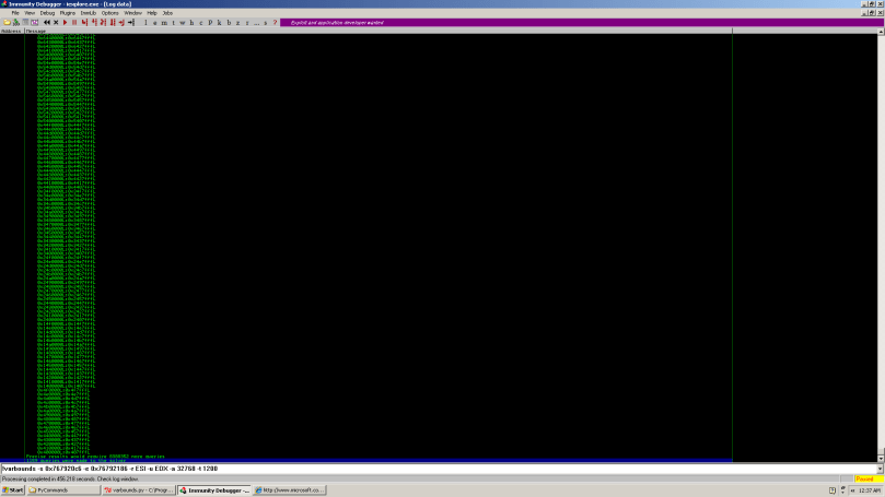
Once this code has run the array sat_ranges contains a list of ranges. In each of these ranges there is at least one valid output value that could potentially end up in v given the correct input values. The larger we set bucket_size the fewer queries we require in this first phase to discover our candidate ranges but the more coarse grained our initial results are. The following screenshot shows an analysis of our earlier code using a bucket size of 32768.

Coarse analysis searching for candidate ranges

1159 queries were required to discover 256 candidate ranges with total run time at 456 seconds. While these results are still far from giving us exact ranges for v (8388352 queries away in fact, which is still far too many to be practical) a definite pattern has emerged in the output values. This pattern is of course an artefact of the logical instructions found in the instruction sequence and we can see quite clearly in the above screen shot all our valid ranges are of the form 0xY4X00000:0xY4X07FFF for all X, Y in [1,..,9]. A quick glance over the instructions involved in the code sequence is enough to indicate that if we can resolve the valid indexes into any of these ranges then the same indexes will be valid for the other ranges.

The script varbounds.py also allows us to specify the initial lower and upper bounds for the ranges so we can use that to investigate a particular range.

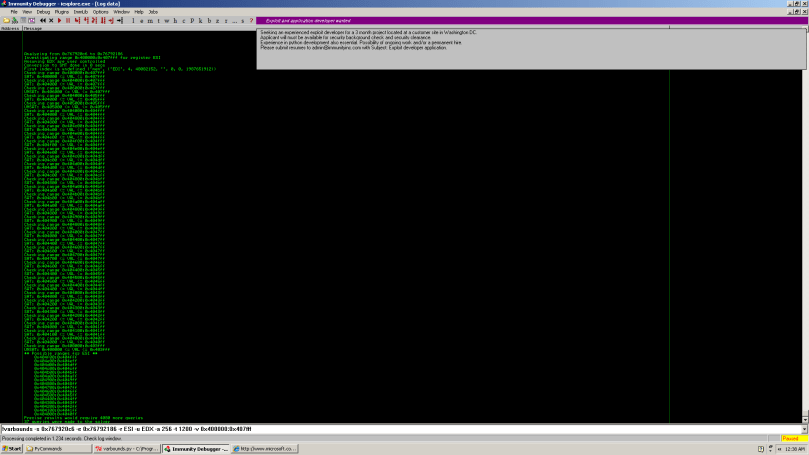
Here we check the 0x0x400000:407fff range

Now we’re starting to get somewhere! By setting the bucket size to 256 and querying the range 0x400000:0x407fff we’ve managed to reduce our potential valid results to living within 16 different buckets of size 256. All this with only 37 queries to the solver and a run time of just over a second. The reason for so few queries is essentially that large ranges were proved unsatisfiable meaning we didn’t have to split/investigate their sub-ranges. In order to discover the exact values that are possible within these ranges we need to take one more step; instead of querying ranges we need to query for concrete values within these ranges as initially proposed. The difference now is that we have reduced our untenable 2**32 queries to a mere 4000 or so.

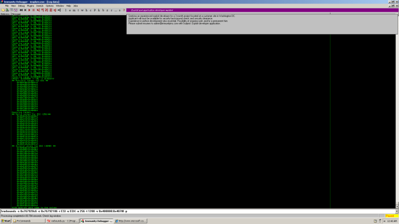
(In the following screenshot the -p option tells the script to use precise queries instead of ranges. The ranges under ** Valid values for ESI ** were constructed by individual queries to the values within these ranges and then merging the ranges after the fact to make the results easier to read)

Discovering the exact values that are possible within the range 0x400000:0x407fff

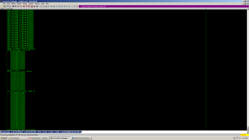
In the end you can see that we have proven there are exactly 256 possible valid values from that initial large range of size 32768. Precise results required 4133 queries which only took 87 seconds to complete. At this point we can extrapolate our results back to the other ranges and come up with a pattern we know any result in ESI will match. It is 0xY4X4Zc0 to 0xY4X4Zcf for all X, Y, Z in [0,..,9].

A quick test on another range confirms this pattern.

Confirming our byte pattern holds for the other ranges

Improving the above solution with abstract interpretation

So for the above test case the results are pretty cool. It is of course easy to think of examples where blindly applying this technique will result in failure to reduce the initial problem of a large potential output space. Consider any sequence of instructions built purely from arithmetic instructions like add, mul, div etc. In this case the binary search would simply split the full output range into a sequence of bucket sized ranges without actually removing any of them as all values are possible given at least one free input variable.

Another pretty obvious point is that by ignoring the semantics of logical operators we are effectively ignoring an even simpler way to perform the initial filtering. In our solution we blindly convert the initial instruction sequence to equations in our SMT solver and then entirely ignore the original instructions for the remainder of our task. Much like the above case we are losing valuable information in doing so. Take the instruction and eax, 0xffff. If such an instruction appears right before the value in eax is moved into our output register then an analysis with the ability to include information on logical operator semantics could pre-limit its search to values in the 0xffff range. A very simple application of abstract interpretation could drastically reduce the number of cases where we need to go to a solver at all by maintaining information on the state of each bit for each register or memory location in play. With an abstract domain consisting of {MUST_BE_SET, CANT_BE_SET, MIGHT_BE_SET} and abstract versions of and, or, xor etc. we could easily propagate the required information e.g. MUST_BE_SET ^ CANT_BE_SET => CANT_BE_SET, MUST_BE_SET ^ MUST_BE_SET => MUST_BE_SET, MUST_BE_SET ^ MIGHT_BE_SET => MIGHT_BE_SET and so on. I haven’t thought this one through entirely and I’m sure there’s a nicer way to present the theory but merging information gained from abstract interpretation into solutions with SMT solving is, in my opinion, one of the most powerful approaches to program analysis at the moment.

A third instruction category worth considering is conditional jumps. By their nature every conditional jump imposes constraints on the path in which it occurs. If it is taken the positive constraint holds, otherwise its negation holds. Once again it is obvious that by ignoring these constraints at a higher level than SMT equations we risk pointless queries to the solver but I haven’t considered the problem enough to come up with a good lightweight abstract analysis. The emphasis here being on ‘lightweight’ as if the solution is more expensive than running the solver then it isn’t worth it.

Scalability

One interesting question posed to me about this script is ‘How does it compare to simply running the code and iterating over the possible input values?’. The honest answer is that I have no metrics on that approach to compare it with. What I would say however is that practically implementing that kind of solution for longer program paths involving memory accesses is likely to be no walk in the park either. As mentioned earlier, each run in such a solution is going to have to restore a ‘snapshot’ of some kind and will require exactly 2^w_0 * … * 2^w_n-1 iterations. The question then becomes ‘How does the solvers running time scale with the number of input variables and their width?’. Again my answer is really the same in that I haven’t ran enough experiments to come to any valid conclusions yet. I would imagine that in the worst case the scaling is just as bad given the nature of the problem but that the average case is far better. Gathering some decent stats on this is actually my next intended project when I get some free time.

Conclusion

1. If you have a specific question you need answering then dealing with annoying instruction sequences doesn’t have to be a nightmare. Solvers. Use them.
2. Solvers. Don’t use them for everything. There’s a world of other awesome program analysis techniques and tools out there than in many situations complement theorem provers and decision procedures very nicely and in other cases can give far superior results. Also, as in the above situation there’s always room for a healthy amount of human interaction and guidance.

Validity, Satisfiability and Code Semantics

In a recent post to DD I mentioned some interesting features that will be available in Immunity Debugger 2.0. These features rely on a translation layer from x86 code to SMT formulae that Pablo constructed as part of his work on DEPLIB 2.0. In the past few weeks I got some time to put together a few scripts for ID that replicate some of the more useful tasks that we can use a solver for. In this post I am going to elaborate on one such script which is designed to find ROP gadgets meeting user specified conditions.

find_gadget.py is a relatively simple piece of software which is a testament to Pablo’s API development, the Python programming language and, I think quite importantly, the suitability of mathematical logic for reasoning about machine code. This final point is of course unsurprising but it provides good motivation when considering the merits of abstracting x86 code to more logical/mathematical representations for analysis.

We begin our gadget search by running gadgets.py. Currently this script finds any instruction sequence ending in a ret instruction (with support for pop REG/jmp REG etc. in the works). This takes about 360 seconds to run on QuickTimeAuthoring.qtx (2.16MB) and finds 80,000 candidate gadgets. For now no further analysis is done on these gadgets but we’re working on some fun stuff in that area.

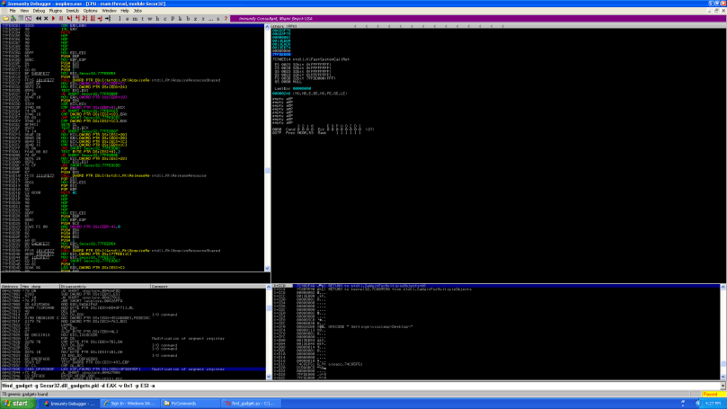
At this point we can use find_gadget.py to search the candidate gadgets for one that meets whatever semantics we have in mind. For now the semantics are specified via the -d, -n and -v/-s options, i.e. DESTINATION RELATION SOURCE/VALUE. For example, to represent EAX <= [EBX+24] we would use -d EAX -n <= -s [EBX+24]. (This is a little cumbersome and not as flexible as one might like so we built a BNF grammar based on pyparsing that allows for arbitrary semantics to be specified as constraints and that should be swapped in pretty soon.) The full set of arguments are shown in this screenshot:

Arguments to find_gadget.py

Once we have specified our arguments the script gets on with the fun part. Our algorithm is as follows:


for gadget in candidiate_gadgets:
    sa = SequenceAnalyzer(reg_model, flag_model, mem_model) # 1
    sa.analyze(gadget.addr, gadget.depth) # 2
    
    if relation == '=':
         rel_expr = sa.solver.eqExpr(dest, src) # 3
    elif relation == '<=':
         ...

    preserve_expr = None
    if preserve_regs != None: # 4
         for reg in preserve_regs:
              eq_expr = sa.solver.eqExpr(sa.regs_before[reg], sa.regs_after[reg])
              preserve_expr = sa.solver.boolAndExpr(preserveExpr, eq_expr)
        rel_expr = sa.solver.boolAndExpr(rel_expr, preserve_expr)

    res = sa.solver.queryFormula(rel_expr) # 5
    if generic_gadgets_only:
         if res == VALID:
              # VALID GADGET FOUND
     else:
          if res == SATISFIABLE:
              # SATISFIABLE GADGET FOUND

#1 Modelling registers, flags and memory
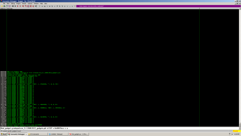
One of the arguments you may have noticed to the script is -c. This argument tells the script that we want to look for ‘context specific’ gadgets that satisfy our semantics when current values in registers, memory and flags are taken into account. The alternative is to look for generic gadgets that will meet the required semantics regardless of the context e.g. inc eax will only set eax to 0 if it previously contained -1 while xor eax, eax will always set it to zero. We’ll discuss this a little more on point #5.

#2 Gadgets to equations
The main coding effort in building this framework was building a transformer for each x86 instruction into the domain of our theorem prover. This requires one to encode accurately the semantics of the instruction over flags, registers and memory and is the backbone of any tool that reasons about assembly code using a solver. This long and drawn out functionality is hidden behind the analyze function which iterates over each instruction and updates the solver state. Once this has completed our solver internally has an accurate representation of the gadgets semantics in the form of several equations.

# 3 & # 4 Adding our gadget constraints
Once one has a representation of a sequence of instructions as equations the next step is typically to append some further constraints derived from the task at hand and then query the solver to determine if they are valid or satisfiable, and if so, to retrieve an input that makes it so. In our case our constraints simply specify a relation between an output register/memory location and an input register/memory location or a constant. We also allow the user to specify a number of registers that the gadget should preserve. We end up with a formula specifying something like (ESP_after == EAX_before+4 AND EBX_after == EBX_before), which is essentially a stack swap with the buffer pointed to by EAX and preserving the EBX register.

# 5 Context specific vs. generic gadgets
After encoding our constraints as a formula in steps #3 and #4 we can then query the solver to determine the status of these constraints in the context of the gadget encoding constructed in step #2. What do we mean by ‘status’? Well, when considering the SAT problem a formula can either be valid, invalid, satisfiable or unsatisfiable. A formula is satisfiable if there exists an assignment to free variables that makes it true and is unsatisfiable otherwise. A formula is valid if its negation is unsatisfiable or invalid otherwise. In other words, a formula is valid if any variable assignment makes it true. Why is this important? If we’re looking for generic gadgets then we want them to meet our constraints regardless of the context, therefore we leave all memory locations, registers and flags free and require that our constraints are VALID in the context of the gadget. That is, there exists no assignment to the memory locations, registers and flags that would result in the gadget not meeting our constraints.

The next few screenshots show some usage examples.

A generic gadget to set EAX to 1
A generic gadget to set EAX to 1 while preserving ESI
Finding multiple gadgets to achieve the same result

find_gadget.py is a very simple script but at the same time can find some very complicated instruction sequences in a short amount of time. In particular it can find tricky stack swapping gadgets and can process about 200,000 gadgets in 3 hours, which is probably a bit quicker than doing it by hand. In some upcoming posts I’ll elaborate a bit more on what can be done with the x86 -> SMT transformer -> solver code. For an idea of some of the things we’re hoping to implement many of the papers published in the last few years on symbolic execution and derived techniques are a good starting point and quite a few are linked from the Practical Software Verification Wiki

Applying Taint Analysis and Theorem Proving to Exploit Development

Last week I spoke at REcon on the above topic. The slides can be found here. The abstract for this talk is as follows:

As reverse engineers and exploit writers we spend much of our time trying to illuminate the relationships between input data, executed paths and the values we see in memory/registers at a later point. This work can often be tedious, especially in the presence of extensive arithmetic/logical modification of input data and complex conditions.

Using recent (and not so recent) advances in run-time instrumentation we can go a long way towards automating the process of tracking input data and its effects on execution. In this talk we will discuss possible approaches to solving this problem through taint analysis. The solutions we will discuss are useful in many scenarios e.g. determining the set of conditional jumps under our control, discovering buffers in memory that are useful for injecting shellcode, tracking parameters to potentially insecure function calls, discovering ‘bad bytes’ for exploits and so on.

Building on this we will delve into the construction of logical formulae expressing the relationships between input and data in memory and ways in which these formulae can be manipulated and solved for interesting results. Depending on how we manipulate the initial formulae we can use theorem provers to automatically solve many problems e.g. ‘unraveling’ arithmetic/logical modifications on input, generating inputs that trigger specific paths, discovering the bounds on given variables and so forth.

I will update this post whenever the REcon videos etc go online. In the meantime I should probably finish at least one of the 5 or so blog posts in a semi-complete state 😛