This post is the first of a two part discussion in which we’ll tackle the title problem with some scripts on top of Immunity Debugger 2.0. To begin lets pose the question as follows: ‘Given an output register or memory location v, of width w, and a set of input registers/memory locations (x_0, w_0), …, (x_n-1, w_n-1) what are the possible values for v after the execution of a sequence of n instructions i_0, i_1, … i_n-1‘. Lets call this sequence p representing any concrete path through a program. Before we continue it may be worth your while to think about some solutions to this problem given whatever tools and techniques you think appropriate.
The most primitive solution is probably to just run the code and iterate over all possible combinations of input variables. This will require exactly 2^w_0 * … * 2^w_n-1 runs and with a running time exponential the number of input variables. Presuming we only want to run our variable range analysis on a specific sub-path then for this solution we need a way to snapshot a process and re-run the sub-path multiple times or, if feasible, re-run the entire path and enable the analysis for the required sub-path.
Lets now presume we have at our disposal a method of converting p into a formula F(p) interpretable by an SMT solver that gives the precise semantics of p. Given what we know about SMT solvers one obvious solution to the above problem immediately presents itself. By creating the conjunction of F(p) with a formula expressing v := x for each x in the range 0 to 2^w-1 we can, with 2^w-1 queries of our solver, determine the full range of possible values for v, those x values resulting in a satisfiable formula, as well as the assignments to input variables that result in each value.
How long will this many queries take to run? Naturally this will be a factor of n and the complexity of the instructions in p (due to the relative solving costs for linear vs non-linear arithmetic and so on) but let’s chose an instruction sequence and do some testing. The following instruction sequence was chosen as it is short enough to serve as a good example but arithmetically complex enough that the potential range of values for ESI at 0x76792186 require some manual labour to figure out.

The input variables to this sequence are EDX and ECX and the output variable we are interested in is ESI (although we could of course look for results for any variable written to during this sequence). Now it’s time to start thinking about our algorithm a little more. For certain output values over this instruction sequence our solving code can hit upwards of 6000 queries a minute but doing this 2^32 times is still going to take a prohibitively long time to finish. Not to mention the fact that we’ll want to run this solution on much longer instruction sequences in the future.
The approach I decided to take here was to try to divide the possible output values into ranges and try to weed out entire ranges of unsatisfiable output values at once by constructing queries like v >= LOWER_BOUND AND v <= UPPER_BOUND. If such a formula is satisfiable then we can conclude that within the range LOWER_BOUND:UPPER_BOUND is at least one output value that can be achieved given the correct input.
Effectively this results in a binary search of the output value space. In the best case scenario the largest ranges possible are proven to be unsatisfiable, or in other words no possible output value lies within that range. e.g. If our range is 0:2**32-1 and we split it in two to query the ranges 0:(2**32-1)/2 and (2**32-1)/2 + 1: 2**32-1 and discover that the first range gives an unsatisfiable result then we have immediately removed 2**32/2 potential output values that we may have otherwise had to investigate. The algorithm is essentially:
lower = 0
upper = 2**32 - 1

ranges = [(lower, upper)]
while len(ranges) > 0:
    lower, upper = ranges.pop()
    query = create_range_query(lower, output_register, upper)
    if solver.isSatisfiable(query):
        diff = lower - upper
        if diff <= bucket_size:
            sat_ranges.append((lower, upper))
        else:
            half = diff/2
            ranges.append(lower, lower + half)
            ranges.append(lower + half + 1, upper)
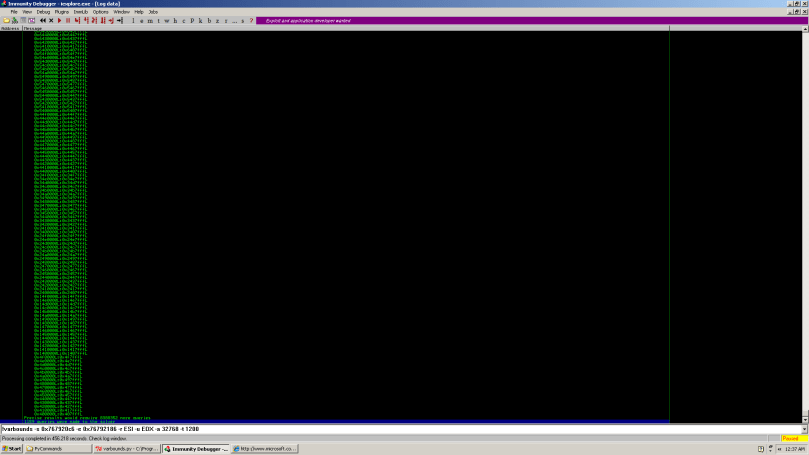
Once this code has run the array sat_ranges contains a list of ranges. In each of these ranges there is at least one valid output value that could potentially end up in v given the correct input values. The larger we set bucket_size the fewer queries we require in this first phase to discover our candidate ranges but the more coarse grained our initial results are. The following screenshot shows an analysis of our earlier code using a bucket size of 32768.

1159 queries were required to discover 256 candidate ranges with total run time at 456 seconds. While these results are still far from giving us exact ranges for v (8388352 queries away in fact, which is still far too many to be practical) a definite pattern has emerged in the output values. This pattern is of course an artefact of the logical instructions found in the instruction sequence and we can see quite clearly in the above screen shot all our valid ranges are of the form 0xY4X00000:0xY4X07FFF for all X, Y in [1,..,9]. A quick glance over the instructions involved in the code sequence is enough to indicate that if we can resolve the valid indexes into any of these ranges then the same indexes will be valid for the other ranges.
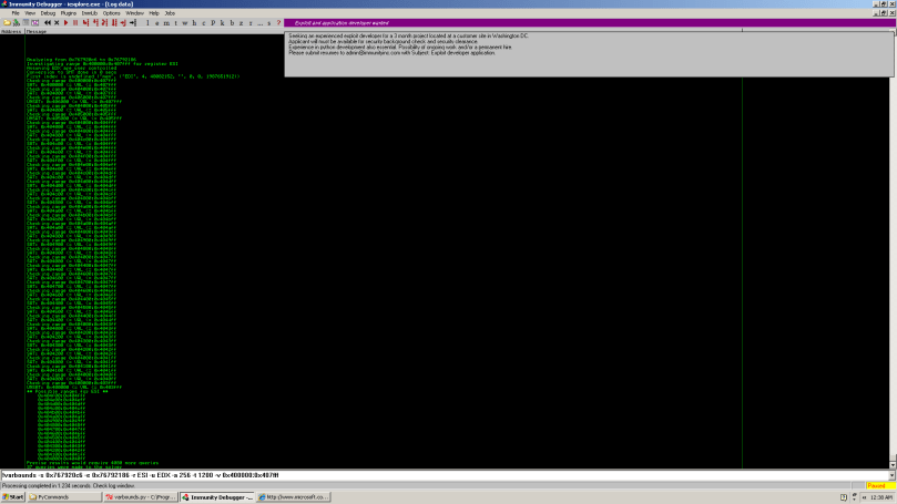
The script varbounds.py also allows us to specify the initial lower and upper bounds for the ranges so we can use that to investigate a particular range.

Now we’re starting to get somewhere! By setting the bucket size to 256 and querying the range 0x400000:0x407fff we’ve managed to reduce our potential valid results to living within 16 different buckets of size 256. All this with only 37 queries to the solver and a run time of just over a second. The reason for so few queries is essentially that large ranges were proved unsatisfiable meaning we didn’t have to split/investigate their sub-ranges. In order to discover the exact values that are possible within these ranges we need to take one more step; instead of querying ranges we need to query for concrete values within these ranges as initially proposed. The difference now is that we have reduced our untenable 2**32 queries to a mere 4000 or so.
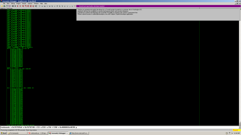
(In the following screenshot the -p option tells the script to use precise queries instead of ranges. The ranges under ** Valid values for ESI ** were constructed by individual queries to the values within these ranges and then merging the ranges after the fact to make the results easier to read)

In the end you can see that we have proven there are exactly 256 possible valid values from that initial large range of size 32768. Precise results required 4133 queries which only took 87 seconds to complete. At this point we can extrapolate our results back to the other ranges and come up with a pattern we know any result in ESI will match. It is 0xY4X4Zc0 to 0xY4X4Zcf for all X, Y, Z in [0,..,9].
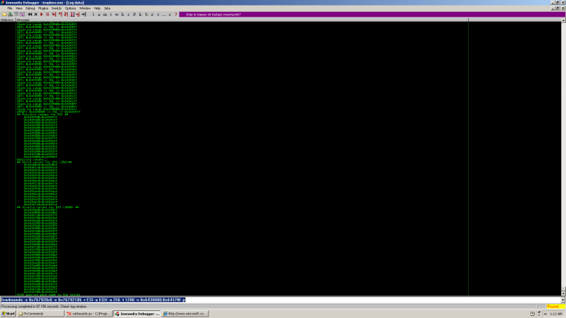
A quick test on another range confirms this pattern.

Improving the above solution with abstract interpretation
So for the above test case the results are pretty cool. It is of course easy to think of examples where blindly applying this technique will result in failure to reduce the initial problem of a large potential output space. Consider any sequence of instructions built purely from arithmetic instructions like add, mul, div etc. In this case the binary search would simply split the full output range into a sequence of bucket sized ranges without actually removing any of them as all values are possible given at least one free input variable.
Another pretty obvious point is that by ignoring the semantics of logical operators we are effectively ignoring an even simpler way to perform the initial filtering. In our solution we blindly convert the initial instruction sequence to equations in our SMT solver and then entirely ignore the original instructions for the remainder of our task. Much like the above case we are losing valuable information in doing so. Take the instruction and eax, 0xffff. If such an instruction appears right before the value in eax is moved into our output register then an analysis with the ability to include information on logical operator semantics could pre-limit its search to values in the 0xffff range. A very simple application of abstract interpretation could drastically reduce the number of cases where we need to go to a solver at all by maintaining information on the state of each bit for each register or memory location in play. With an abstract domain consisting of {MUST_BE_SET, CANT_BE_SET, MIGHT_BE_SET} and abstract versions of and, or, xor etc. we could easily propagate the required information e.g. MUST_BE_SET ^ CANT_BE_SET => CANT_BE_SET, MUST_BE_SET ^ MUST_BE_SET => MUST_BE_SET, MUST_BE_SET ^ MIGHT_BE_SET => MIGHT_BE_SET and so on. I haven’t thought this one through entirely and I’m sure there’s a nicer way to present the theory but merging information gained from abstract interpretation into solutions with SMT solving is, in my opinion, one of the most powerful approaches to program analysis at the moment.
A third instruction category worth considering is conditional jumps. By their nature every conditional jump imposes constraints on the path in which it occurs. If it is taken the positive constraint holds, otherwise its negation holds. Once again it is obvious that by ignoring these constraints at a higher level than SMT equations we risk pointless queries to the solver but I haven’t considered the problem enough to come up with a good lightweight abstract analysis. The emphasis here being on ‘lightweight’ as if the solution is more expensive than running the solver then it isn’t worth it.
Scalability
One interesting question posed to me about this script is ‘How does it compare to simply running the code and iterating over the possible input values?’. The honest answer is that I have no metrics on that approach to compare it with. What I would say however is that practically implementing that kind of solution for longer program paths involving memory accesses is likely to be no walk in the park either. As mentioned earlier, each run in such a solution is going to have to restore a ‘snapshot’ of some kind and will require exactly 2^w_0 * … * 2^w_n-1 iterations. The question then becomes ‘How does the solvers running time scale with the number of input variables and their width?’. Again my answer is really the same in that I haven’t ran enough experiments to come to any valid conclusions yet. I would imagine that in the worst case the scaling is just as bad given the nature of the problem but that the average case is far better. Gathering some decent stats on this is actually my next intended project when I get some free time.
Conclusion
1. If you have a specific question you need answering then dealing with annoying instruction sequences doesn’t have to be a nightmare. Solvers. Use them.
2. Solvers. Don’t use them for everything. There’s a world of other awesome program analysis techniques and tools out there than in many situations complement theorem provers and decision procedures very nicely and in other cases can give far superior results. Also, as in the above situation there’s always room for a healthy amount of human interaction and guidance.

A possible improvement still using a solver could be to query each bit for VALID 0s and 1s.
8bits example:
Start with
UPPER_RANGE = 11111111 and
LOWER_RANGE = 00000000.
and we need to process:
AND AL, 0x3f
OR AL, 0x10
Set 0 on the UPPER_RANGE bit if it returns VALID for:
QUERY AL & onebitatthetime == 0
Set 1 on the LOWER_RANGE if it returns VALID for:
QUERY AL & onebitatthetime != 0
The result in this case would leave UPPER_RANGE = 00111111 and LOWER_RANGE = 00010000, thus narrowing the range down and it takes into consideration bit operations.
PD: I *do* agree with your conclusions and I really enjoy reading your blog 🙂
pablo.
Good point 😀
I’ll add that when I’m back (unless you already have. If so commit to SVN :P)
Hi Sean,
Would not it be better to use abstract interpretation (interval analysis) whit SMT Solve ?
Translate the asm code in formulaes and this in transfer functions for interval analysis …
I am researching these issues with a framework for static analysis.
I would like to talk to you. send me a mail.
Regards,
Hi Ivan,
Depends on what you mean by ‘better’. In almost all ways, yes it could be quite a lot better. In terms of time/speed of implementation though, probably not. This code came about basically by me wanting to attack the problem with our x86 -> SMT formula translation library and to see how a purely SMT based approach would fare. The solution is a couple of hundred lines of very basic Python wrapping the SMT library’s API. So in terms of the amount of time/effort for me to implement and test the solution this is the best approach. As for the resulting script it can be slow, especially if we have more than one undefined input variable of size 32 bits or greater. It is however quite usable and can deal with pretty complex sets of instructions accurately.
So what about scalability? In this regard we could definitely do better. Undefining two or more registers for the example in the post results in some prohibitively long running times. Some sort of abstract analysis to limit the ranges that need to be considered by the solver could help deal with this.
One abstract domain is, as you mention, is integer intervals. Another is the slightly simpler, but less accurate, bitwise three-valued logical domain mentioned in the post. There are a wide variety of others varying in accuracy and complexity. A solid solution should at least consider one (and probably more) of these domains but will also require an extra coding effort. For now ImmDbg 2.0 doesn’t provide support for an abstract interpretation based solution but it is something I have in mind and would definitely like to see/do. There’s more effort involved in this than you might think as there is quite a lot of ground work to be layed e.g. from what I can tell the ImmDbg API doesn’t even do proper tracking of local variables, then you also need to consider alias analysis, loops, intrerprocedural analysis and so on. It’s not a huge amount of effort but it was more than I felt like doing for this particular post. (Note the ‘Part 1’ though ;))